Poincaré maps

In this example, we shall illustrate how to construct a Poincaré map associated with the surface of section $x=0$, $\dot x>0$, for $E=0.1025$ for the Hénon-Heiles system. This is equivalent to find the roots of an appropriate function g(dx, x, params, t). We illustrate the implementation using many initial conditions (Monte Carlo like implementation), and then compare the results with the use of jet transport techniques.

Monte Carlo simulation

The Hénon-Heiles system is a 2-dof Hamiltonian system used to model the (planar) motion of a star around a galactic center. The Hamiltonian is given by $H = (p_x^2+p_y^2)/2 + (x^2+y^2)/2 + \lambda (x^2y-y^3/3)$, from which the equations of motion can be obtained; below we concentrate in the case $\lambda=1$.

# Hamiltonian
V(x,y) = 0.5*( x^2 + y^2 )+( x^2*y - y^3/3)
H(x,y,p,q) = 0.5*(p^2+q^2) + V(x, y)
H(x) = H(x...)

# Equations of motion
function henonheiles!(dq, q, p, t)
    x, y, px, py = q
    dq[1] = px
    dq[2] = py
    dq[3] = -x-2y*x
    dq[4] = -y-(x^2-y^2)
    nothing
end

We set the initial energy, which is a conserved quantity; x0 corresponds to the initial condition, which will be properly adjusted to be in the correct energy surface.

# initial energy and initial condition
const E0 = 0.1025
x0 = [0.0, 0.45335, 0.0, 0.0]

In order to be able to generate (random) initial conditions with the appropriate energy, we write a function px, which depends on x, y, py and the energy E, that returns the value of px>0 for which the initial condition [x, y, px, py] has energy E:

# px: select px0>0 such that E=E0
px(x, E) = sqrt(2(E-V(x[1], x[2]))-x[4]^2)

# px!: in-place version of px; returns the modified initial condition `x0`
function px!(x, E)
    mypx = px(x, E)
    x[3] = mypx
    return x
end

# run px!
px!(x0, E0)

4-element Vector{Float64}:
 0.0
 0.45335
 0.24817464176177093
 0.0

Let's check that the initial condition x0 has actually energy equal to E0, up to roundoff accuracy:

H(x0)

0.1025

The scalar function g, which may depend on the time t, the vector of dependent variables x, the velocities dx, and perhaps some parameters params, following again the convention of DifferentialEquations.jl, defines the surface of section by means of the condition $g(dx, x, params, t) = 0$. Internally, the function g is assumed to return a Tuple{Bool, Taylor1{T}}, where T corresponds to eltype(x[1]) (x::Vector{Taylor1{T}}). In the particular case that the user wishes to discard a particular crossing (or crossings), the function g must return a false value, as will be illustrated below.

For the present example, we are looking for crossings through the surface $x=0$, which corresponds to x[1]==0, restricting the crossings to satisfy $\dot x > 0$. i.e., x[3]>0. We thus define the function g as

# x=0, px>0 section
function g(dx, x, p, t)
    px_ = constant_term(x[3])
    # if px > 0...
    if px_ > zero(px_)
        return (true, x[1])
    else
        #otherwise, discard the crossing
        return (false, x[1])
    end
end

We initialize some auxiliary arrays, where we shall save the solutions:

# number of initial conditions
nconds = 100
tvSv = Vector{Vector{Float64}}(undef, nconds)
xvSv = Vector{Matrix{Float64}}(undef, nconds)
gvSv = Vector{Vector{Float64}}(undef, nconds)
x_ini = similar(x0)

We generate nconds random initial conditions in a small neighborhood around x0 and integrate the equations of motion from t0=0 to tmax=135, using a polynomial of order 25 and absolute tolerance 1e-25:

using TaylorIntegration

for i in 1:nconds
    rand1 = rand()
    rand2 = rand()
    x_ini .= x0 .+ 0.005 .* [0.0, sqrt(rand1)*cos(2pi*rand2), 0.0, sqrt(rand1)*sin(2pi*rand2)]
    px!(x_ini, E0)   # ensure initial energy is E0

    sol_i = taylorinteg(henonheiles!, g, x_ini, 0.0, 135.0,
        25, 1e-25, maxsteps=30000);
    tvSv[i] = vcat(0.0, sol_i.t)
    xvSv[i] = vcat(transpose(x_ini), sol_i.x)
    gvSv[i] = vcat(0.0, sol_i.gresids)
end

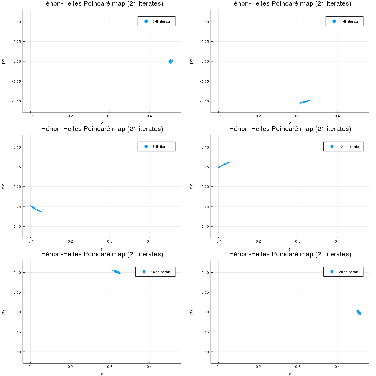
We generate an animation with the solutions

using Plots
poincare_anim1 = @animate for i=1:21
    scatter(map(x->x[i,2], xvSv), map(x->x[i,4], xvSv), label="$(i-1)-th iterate",
        m=(1,stroke(0)), ratio=:equal)
    xlims!(0.09,0.51)
    ylims!(-0.11,0.11)
    xlabel!("y")
    ylabel!("py")
    title!("Hénon-Heiles Poincaré map (21 iterates)")
end

Plots.Animation("/tmp/jl_MPfwiC", ["000001.png", "000002.png", "000003.png", "000004.png", "000005.png", "000006.png", "000007.png", "000008.png", "000009.png", "000010.png"  …  "000012.png", "000013.png", "000014.png", "000015.png", "000016.png", "000017.png", "000018.png", "000019.png", "000020.png", "000021.png"])

gif(poincare_anim1, "poincareanim1.gif", fps = 2)

[ Info: Saved animation to /home/runner/work/TaylorIntegration.jl/TaylorIntegration.jl/docs/build/poincareanim1.gif

Jet transport

Now, we illustrate the use of jet transport techniques in the same example, that is, we propagate a neighborhood around x0, which will be plotted in the Poincaré map. We first define the vector of small increments of the phase space variables, xTN; we fix the maximum order of the polynomial expansion in these variables to be 4. Then, x0TN is the neighborhood in the 4-dimensional phase space around $x0$.

xTN = set_variables("δx δy δpx δpy", numvars=length(x0), order=4)
x0TN = x0 .+ xTN

As it was shown above, $x0$ belongs to the energy surface $H(x0) = E_0 = 0.1025$; yet, as it was defined above, the set of phase space points denoted by x0TN includes points that belong to other energy surfaces. This can be noticed by computing H(x0TN)

H(x0TN)

 0.1025 + 0.2478237775 δy + 0.24817464176177093 δpx + 0.9533499999999999 δx² + 0.046650000000000025 δy² + 0.5 δpx² + 0.5 δpy² + 1.0 δx² δy - 0.3333333333333333 δy³ + 𝒪(‖x‖⁵)

Clearly, the expression above may contain points whose energy is different from E0. As it was done above, we shall fix the px component of x0TN so all points of the neighborhood are in the same energy surface.

px!(x0TN, E0) # Impose that all variations are on the proper energy shell!
H(x0TN)

 0.1025 - 5.551115123125783e-17 δy² - 5.551115123125783e-17 δy³ - 1.7763568394002505e-15 δx² δy² - 4.440892098500626e-16 δy⁴ + 8.881784197001252e-16 δy² δpy² + 𝒪(‖x‖⁵)

We notice that the coefficients of all monomials whose order is not zero are very small, and the constant_term is E0.

In order to properly handle this case, we need to extend the definition of g to be useful for Taylor1{TaylorN{T}} vectors.

#specialized method of g for Taylor1{TaylorN{T}}'s
function g(dx::Array{Taylor1{TaylorN{T}},1}, x::Array{Taylor1{TaylorN{T}},1},
        p, t) where {T<:Number}
    px_ = constant_term(constant_term(x[3]))
    if px_ > zero( T )
        return (true, x[1])
    else
        return (false, x[1])
    end
end

We are now set to carry out the integration.

solTN = taylorinteg(henonheiles!, g, x0TN, 0.0, 135.0, 25, 1e-25, maxsteps=30000);

We define some auxiliary arrays, and then make an animation with the results for plotting.

#some auxiliaries:
tvTN, xvTN, tvSTN, xvSTN, gvSTN = solTN.t, solTN.x, solTN.tevents, solTN.xevents, solTN.gresids
xvSTNaa = Array{Array{TaylorN{Float64},1}}(undef, length(tvSTN)+1 );
xvSTNaa[1] = x0TN
for ind in 2:length(tvSTN)+1
    whatever = xvSTN[ind-1,:]
    xvSTNaa[ind] = whatever
end
tvSTNaa = union([zero(tvSTN[1])], tvSTN);

myrnd  = 0:0.01:1
npoints = length(myrnd)
ncrosses = length(tvSTN)
yS = Array{Float64}(undef, ncrosses+1, npoints)
pS = Array{Float64}(undef, ncrosses+1, npoints)

myrad=0.005
ξy = @. myrad * cos(2pi*myrnd)
ξp = @. myrad * sin(2pi*myrnd)

for indpoint in 1:npoints
    yS[1,indpoint] = x0[2] + ξy[indpoint]
    pS[1,indpoint] = x0[4] + ξp[indpoint]
    mycond = [0.0, ξy[indpoint], 0.0, ξp[indpoint]]
    for indS in 2:ncrosses+1
        temp = evaluate(xvSTNaa[indS], mycond)
        yS[indS,indpoint] = temp[2]
        pS[indS,indpoint] = temp[4]
    end
end

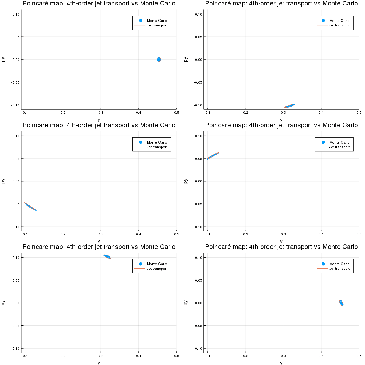
poincare_anim2 = @animate for i=1:21
    scatter(map(x->x[i,2], xvSv), map(x->x[i,4], xvSv), marker=(:circle, stroke(0)),
        markersize=0.01, label="Monte Carlo")
    plot!(yS[i,:], pS[i,:], width=0.1, label="Jet transport")
    xlims!(0.09,0.51)
    ylims!(-0.11,0.11)
    xlabel!("y")
    ylabel!("py")
    title!("Poincaré map: 4th-order jet transport vs Monte Carlo")
end

Plots.Animation("/tmp/jl_l7MCkm", ["000001.png", "000002.png", "000003.png", "000004.png", "000005.png", "000006.png", "000007.png", "000008.png", "000009.png", "000010.png"  …  "000012.png", "000013.png", "000014.png", "000015.png", "000016.png", "000017.png", "000018.png", "000019.png", "000020.png", "000021.png"])

gif(poincare_anim2, "poincareanim2.gif", fps = 2)

[ Info: Saved animation to /home/runner/work/TaylorIntegration.jl/TaylorIntegration.jl/docs/build/poincareanim2.gif

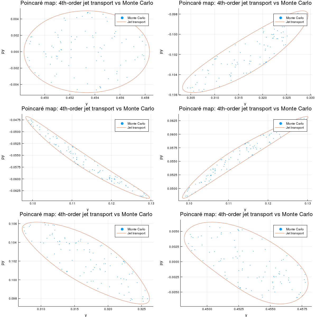
The next animation is the same as before, adapting the scale.

poincare_anim3 = @animate for i=1:21
    scatter(map(x->x[i,2], xvSv), map(x->x[i,4], xvSv), marker=(:circle, stroke(0)),
        markersize=0.1, label="Monte Carlo")
    plot!(yS[i,:], pS[i,:], width=0.5, label="Jet transport")
    xlabel!("y")
    ylabel!("py")
    title!("Poincaré map: 4th-order jet transport vs Monte Carlo")
end

Plots.Animation("/tmp/jl_SvM9Y9", ["000001.png", "000002.png", "000003.png", "000004.png", "000005.png", "000006.png", "000007.png", "000008.png", "000009.png", "000010.png"  …  "000012.png", "000013.png", "000014.png", "000015.png", "000016.png", "000017.png", "000018.png", "000019.png", "000020.png", "000021.png"])

gif(poincare_anim3, "poincareanim3.gif", fps = 2)

[ Info: Saved animation to /home/runner/work/TaylorIntegration.jl/TaylorIntegration.jl/docs/build/poincareanim3.gif